This weekend as a fun project, I thought to hindcast (prediction for the past) through linear discriminant analysis (LDA), if I went for a run on a given day or not, using the Apple Watch data that keeps a track of health and fitness information, encompassing activity levels, sleep patterns, body temperature, heart rate variations etc.

Problem Statement

I decided to implement linear discriminant analysis (LDA) from scratch, I mean capital-S scratch. I won’t even use NumPy, Pandas or Scipy or anything; just pure good 'ol Python with its humble lists, some built-in tools and the first principles of linear algebra and statistics. I've even hand-coded tasks like matrix multiplication, inversion and maximum likelihood estimation from ground up. By the way, this whole endeavour has a street name: 'Not Invented by Me' syndrome, for those who lose sleep over not inventing the wheel themselves. Anyway, a word of caution: don't try this at home since iteration over Python lists is painfully slow, being pointers to objects in noncontiguous memory, or your computer might question its existence and you might question my sanity (truth be told, I sometimes do too), but let’s look how it turned out!

All the code is in notebook here: LDA from scratch

A photo I took while running a trail in Bavaria, Germany.

Implementing LDA, the hard way

The data has been sourced from Apple Health and Nike Run Club. The data was easy to export as Apple Health has a button to export your personal health data locally. The running data is just one binary variable, did I run or not run on that day, but the data was a pain to retrieve. But runners are persistent and stubborn so someone wrote a Python library to extract data from Nike Run Club. Visualising this data as a simple scatterplot, does reveal certain interesting characterstics. To keep things simple, I will use my maximum heart rate recorded throughout the day and active energy burned that is the calories burned when I was physically active to predict whether I went for a run or not.

Figure 1: Average Heart Rate, Active Energy and Wrist Temperature (Blue dots represent the days I ran)

If you look carefully, I have visualised 4 dimensions in this scatterplot. The color represents the binary outcome - whether I ran or did not. The x-axis represents the average heart rate, the y-axis represents the active energy burned, the size of the dots represents the average wrist temperature during the day (scaled relatively). This kind of visualisation is interesting and it can reveal a lot about the interplay of these features. For example, the days I ran intensively, I had a higher average wrist temperature. The day I had a fever, I did not run, I had a very low active energy burned and a high wrist temperature. All of this is visualized below. It is interesting indeed.

Figure 2: Insights from Data

And then I found the decision rule (hyperplane) that separates the classes, visualised as follows: Figure 3: Running data with decision boundary found through LDA

Now, let us dive into the the first principles and mathematics behind LDA which I have implemented. If you are not into mathematics and statistics, you can skip this section.

First Principles and math

Let's simplify the notations for better readability and ease of typing. We denote $k$ as 0 or 1 for "not run" and "run," respectively. $\mathbf{P}[Y_i = k | X_i]$ represents the probability of running or not running given the observation $X_i$, consisting of heart rate and active energy.

$\mathbf{P}[X_i | Y_i = k]$ signifies the likelihood of observing heart rate and active energy $X_i$ given $Y_i = k$, reflecting how these factors are distributed during running or not running. $\mathbf{P}[Y_i = k]$ denotes the prior probability of running or not running irrespective of heart rate and active energy. $\mathbf{P}[X_i]$ stands for the marginal probability of observing evidence $X_i$, calculated by summing over all possible values of $Y_i$ (0 and 1). In essence, it's the unconditional probability of observing evidence $X_i$. With $Y_i$ as a binary variable indicating running ($Y_i = 1$) or not ($Y_i = 0$), and $X_i$ as a vector representing heart rate and active energy, we derive the formula:

The first step is the application of Bayes' rule. In the second step, the denominator is expanded using the law of total probability. The denominator, $\mathbf{P}[X_i]$, is expressed as the sum of the joint probabilities of $X_i$ and $Y_i$ over all possible values of $Y_i$. This is the prior probability of $X_i$. The proportionality in step 3, indicates that the expression is proportional to the product of the likelihood and the prior, with the constant of proportionality being the marginal probability of the heart rate and the active energy $X_i$. Deriving this expression, was precisely the intent behind going through all these steps. The implication is important:

If we know the likelihood $\mathbf{P}[X_i | Y_i = k]$ and the prior $\mathbf{P}[Y_i = k]$, we can find a decision rule $D(X_i)$ as a function of evidence that discriminates between the two classes.

This is the substance of Linear Discriminant Analysis.

ASSUMPTIONS

Now let us keep our tradition and decrease the degree of elegance by starting to assume some distributions for the likelihood and the prior.

• The first assumption considers the likelihood to follow a multivariate Gaussian distribution with mean $\mu_k$ and covariance $\Sigma$, denoted as $X_i | Y_i = k \sim \mathcal{N}(\mu_k, \Sigma_k)$. This translates into the probability density function $f_k(x)$, characterized by the Gaussian formula.

Now the conditional probability of class $k$ given the observation $X_i$ is:

Taking the logarithm of both sides (to make life easier), we get:

• The second assumption is, the prior probability of the $k$th class, $\pi_k$, is determined by the proportion of observations belonging to class $k$ in the training sample, reflecting the frequency of running days relative to total days. With these assumptions in place, the conditional probability of class $k$ given observation $X_i$ can be expressed as $\mathbf{P}[Y_i = k | X_i]$.

• The third assumption is that the covariance matrix is the same for both classes. $\Sigma_k = \Sigma$

FINDING THE HYPERPLANE

With this assumption of equal covariance matrix, we can simplify the likelihood equation as:

Now, we determine which class produces the evidence or observed features with the highest likelihood. An observation is predicted to belong to class 1 if:

In simpler terms, given my heart rate and active energy, I predict that I will go on a run if the above inequality is true—that is, the likelihood of running is higher than the likelihood of not running.

After some algebraic manipulation, we simplify the expression to:

This is the decision rule, we need to implement. It encapsulates the essence of LDA — it finds a hyperplane that maximizes the distance between the means of the classes under the given assumptions.

And we get this beautiful decision boundary: Figure 4: Running data with decision boundary found through LDA

Running the model on test data gives me 100% accuracy. All test observations are either true-positive or true-negative. To be very honest, this was expected as running has a direct causal relationship with maximum heart rate. However, the implementation from ground up was fun!. Another cool thing about LDA is that we can use it to reduce dimensionality. The equation of this decision boundary is a linear combination of the original features, and it effectively represents a one-dimensional subspace within the original 2D space. After projecting all points onto the decision boundary, we obtain a set of 1D coordinates corresponding to their positions on this line. These 1D coordinates can be considered as a reduced-dimensional representation of the original 2D data, capturing the essential information relevant to the decision boundary. The linear projection with slightly modified dataset where I used mean heart rate and active energy for each day is visualised below:

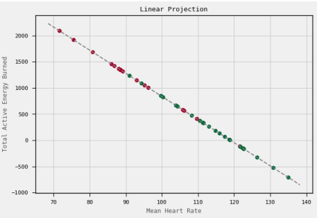Figure 4: Linear Projection found through LDA

That's it. The entire logic and math above is coded from ground up (nobody else’s code and nobody else’s data). All of it is in Jupyter notebook here: LDA from scratch

Citations

1. Fan, J., Li, R., Zhang, C.-H., and Zou, H. (2020). Statistical Foundations of Data Science. CRC Press, forthcoming.
2. Wikipedia. Quadratic Classifier. https://en.wikipedia.org/wiki/Quadratic_classifier
3. Bishop, Christopher M. (2006). Pattern Recognition and Machine Learning. Springer.
4. Jones, Andrew Charles. LDA Explained. https://github.com/rushrukh/explainable_ai_literature